|
Basic Molecular Data
 | Collision rate coefficients
 | Collision rates
maintained by S. Green at NASA GISS. |
| BASECOL database for
ro-vibrational collisional excitation. |
| Collision rates between CO, CS, OCS and HC3N with He and H2 are presented
for temperature up to 100K and up to J=20. The rates are computed by solving quantum mechanical
equations. (from Green & Chapman, 1978ApJS...37..169G) |
| Summaries of theoretical methods and
uncertainties involved in determining collisional rate coefficients are given in books:
-- Roueff, E., 1990, in Molecular Astrophysics, ed. T. W. Hartquist (Cambridge University Press), 232.
-- Flower, E. 1990, in Molecular collisions in the interstellar medium, Cambridge Astrophysics Series (Cambridge: Unversity Press) |
| Ro-vibrational collision rates
of diatomic molecules: Chandra & Sharma, 2001A&A...376..356C. |
| LAMDA database:
energy levels, statistical
weights, Einstein A-coefficients and
collisional rate coefficients of some astrophysically
intersting molecules are given. Collision rates are extrapolated to higher energies
(up to E/k ~ 1000 K). (from Schoier et al.,
2005A&A...432..369S)
 | Rate of collision is  where ncol is the number density of the collision
partners and gamma_ul is the downward
collision rate coefficient (in cm^3s^-1).
gamma_ul is the Maxwellian average of the collision cross section,
sigma, where ncol is the number density of the collision
partners and gamma_ul is the downward
collision rate coefficient (in cm^3s^-1).
gamma_ul is the Maxwellian average of the collision cross section,
sigma,
where k is Boltzmann constant, mu is the reduced mass of the system,
and E is the center-of-mass collision energy. |
| The upward collision rate coefficient
can be derived through detailed balance as
where g is a statistic weight. |
| The collision coefficient rates of collisions with He and H2 at low
gas temperature can be roughly scaled to each other through
and if X is more massive than He and H2, the scaling factor is ~1.4.
This is because the cross section of H2 at J=0
state is equal to that of He. This formula works the best for
O->S substitutions (e.g., HCO+ -> HCS+). The values with H2, J=1 can be larger by factors of 2-5 due
to more interaction potential terms. |
| Uncertainties of collision rate
coefficients:
-- Close-Coupling (CC) method: a few % (work well for low collision energies
and reltively light species);
-- Coupled States (CSt) method: ~10% to a factor of 2;
-- Infinite Order Sudden (IOS)
approximation: up to a order of magnitude.
(the largest source of error is from the
potential surfaces and it is difficult to assess. The most
accurate method is that of Configuration Interaction (CI), but it is
time consuming. Other methods like Hartree-Fock Self-Consisten-field
(SCF), perturbation methods and Density Functional Theory (DFT), all
have its drawbacks. Electron Gas model is outdated, but still in use
in some cases.) |
| How to extrapolate collision rate coefficients from existed data:
| Linear molecules |
| If the basic downward rate coefficients gamma_ L0 (from other levels to
the ground level) are known, then the rate coefficients among
any pairs of levels can be calculated from
where the term in the large parentheses is the Wigner 3-j
symbol. This is valid only in the limit
where the kinetic energy of the colliding molecules is large
compared to the energy splitting of the rotational levels.
This limit can be overcome by multiplying to the part within the
summation with
where  and B0 is the
rotational constant in cm^-1, l is the scattering length in
angstrum (usually l ~ 3 A), mu is the reduced mass of the system
in amu, and T is the kinetic temperature in K. This formula can
be used to exptrapolate down to J=0 for both T and J. and B0 is the
rotational constant in cm^-1, l is the scattering length in
angstrum (usually l ~ 3 A), mu is the reduced mass of the system
in amu, and T is the kinetic temperature in K. This formula can
be used to exptrapolate down to J=0 for both T and J. |
| The basic rate coefficient gamma_L0
can be extended from existed data set in either of two alternative
ways:
# -- use  , in
which y = dEul / kT, and a,b and c are parameters to be determined
from existed data (better over a larger range of energy, and can
be used for other level pairs, with uncertainty within 50%,
typically within 20%); , in
which y = dEul / kT, and a,b and c are parameters to be determined
from existed data (better over a larger range of energy, and can
be used for other level pairs, with uncertainty within 50%,
typically within 20%);
# -- use  to
fit existed data set to determine a, b and c. to
fit existed data set to determine a, b and c. |
| Non-linear molecules |
| No general formula in this case. One needs to inspect the
existed data set and find an approximation function for
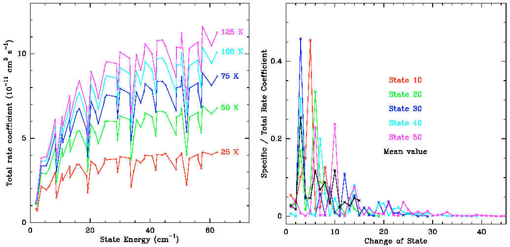
the extrapolation. Here is the example of SO2:
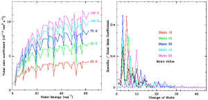
Here the left figure shows the trends of collision rate
coefficients over J and T, the right figure shows the dependence
upon DJ. |
|
|
| Rotational excitation rate coefficients
of HC3N (J=0-50)
with H2 and He
at low temperature (5-100K) are obtained
from extensive quantum (Close Coupling for J<=15) and quasi-classical
(Quasi-Classic Trajectory method for J>15) calculations using new
accurate potential energy surfaces (PES). The rod-like symmetry of the
PES strongly favor even dJ transitions and
efficiently drives large dJ transitions. Rates of
ortho-H2 and para-H2 are similar at the low temperature, due to the
predominance of the geometry effects. Population
inversion is possible with the selective collision pumping in
steady state with H2 density of 10^4-10^6 cm^-3. The collision rate
coefficients are fitted with a formula:
log10( K_J,J'(T)
) = SUM_n=0^4{ a_J,J'^(n)
* x^n }
in which K_J,J'(T) is the rate coefficient
from upper level J to lower level J' at temperature T, a_J,J'^(n) are 5 coefficients (n=0,1,2,3,4)
determined by fitting the accurate results and tabulated in their
electronic table 1A, and x = T^(-1/6). All
the collision rate coefficients can be reproduced from these fitted
formulae. This is their procedure to calculate the collisioin rate
coefficients:
Part 1: calculate the potential energy
surface (PES)
define spatial grids to
sample distance between HC3N-H2 and orientations =>
use the direct parallel code
DIRCCR12 to calculate the PES at each grid point =>
use angular spline to
represent the PES (using a scaling function Sf for larger
distance)
Part 2: dynamic calculation
use MOLSCAT code to perform
close coupling calculations for lower levels (J<=15) =>
use Monte Carlo Quasi-Classic
Trajectory (QCT) method for higher levels (J>15)
Here is a space separated text version of the electronic table 1A: Wernli_2007A+A___464_1147W_tab1a.txt.
(from Wernli et al., 2007A&A...464.1147W) |
| They calculated the rate coefficients among the first 41 rotational levels of the silicon monosulfide (SiS) molecule in its ground vibrational state in collision with para-
and ortho-H. (from Klos & Lique, 2008MNRAS.tmp.1004K)
|
|
| |
|


